Show me the good stuff
pacman::p_load(jsonlite, tidygraph, ggraph, DT, visNetwork, graphlayouts, ggforce,
skimr, tidytext, tidyverse, ggplot2, dplyr, patchwork)As part of the ISSS608-VAA Course in MITB, SMU, Question 1 of the Vast Challenge [Mini Challenge 3] will be addressed as Take-Home Exercise 3.
Q1: Use visual analytics to identify anomalies in the business groups present in the knowledge graph.
pacman::p_load(jsonlite, tidygraph, ggraph, DT, visNetwork, graphlayouts, ggforce,
skimr, tidytext, tidyverse, ggplot2, dplyr, patchwork)mc3_data <- fromJSON("data/MC3.json")mc3_edges <- as_tibble(mc3_data$links) %>%
distinct() %>%
mutate(source = as.character(source),
target = as.character(target),
type = as.character(type)) %>%
group_by(source, target, type) %>%
summarise(weights = n()) %>%
filter(source!=target) %>%
ungroup()mc3_nodes <- as_tibble(mc3_data$nodes) %>%
mutate(country = as.character(country),
id = as.character(id),
product_services = as.character(product_services),
revenue_omu = as.numeric(as.character(revenue_omu)),
type = as.character(type)) %>%
select(id, country, type, revenue_omu, product_services) %>%
distinct(id, country, type, .keep_all = TRUE) #Match for first three columnsCheck for Missing Values
skim(mc3_edges)| Name | mc3_edges |
| Number of rows | 24036 |
| Number of columns | 4 |
| _______________________ | |
| Column type frequency: | |
| character | 3 |
| numeric | 1 |
| ________________________ | |
| Group variables | None |
Variable type: character
| skim_variable | n_missing | complete_rate | min | max | empty | n_unique | whitespace |
|---|---|---|---|---|---|---|---|
| source | 0 | 1 | 6 | 700 | 0 | 12856 | 0 |
| target | 0 | 1 | 6 | 28 | 0 | 21265 | 0 |
| type | 0 | 1 | 16 | 16 | 0 | 2 | 0 |
Variable type: numeric
| skim_variable | n_missing | complete_rate | mean | sd | p0 | p25 | p50 | p75 | p100 | hist |
|---|---|---|---|---|---|---|---|---|---|---|
| weights | 0 | 1 | 1 | 0 | 1 | 1 | 1 | 1 | 1 | ▁▁▇▁▁ |
Clean up Grouped Data (Source)
mc3_edges_clean <- mc3_edges%>%
  # Extract all text within " "
  mutate(source = str_extract_all(source, '"(.*?)"')) %>%
  # Split into separate rows
  unnest(source) %>%
  # Split phrases by comma ignoring leading spaces
  separate_rows(source, sep = ",\\s*") %>%
  mutate(source = str_remove_all(source, '"'))
Checking for duplicates
mc3_edges_clean[duplicated(mc3_edges_clean),]# A tibble: 2,238 × 4
source target type weights
<chr> <chr> <chr> <int>
1 1 Ltd. Liability Co Yesenia Oliver Company Contacts 1
2 1 Swordfish Ltd Solutions Daniel Reese Company Contacts 1
3 6 GmbH & Co. KG Monique Cummings Company Contacts 1
4 6 GmbH & Co. KG Monique Cummings Company Contacts 1
5 Mar de la Luz BV Monique Cummings Company Contacts 1
6 7 Ltd. Liability Co Express Cassidy Sherman Beneficial Owner 1
7 7 Ltd. Liability Co Express Dawn West Beneficial Owner 1
8 7 Ltd. Liability Co Express Hannah Franco Company Contacts 1
9 7 Ltd. Liability Co Express Michael Morrison Beneficial Owner 1
10 7 Ltd. Liability Co Express Nicole Carrillo Beneficial Owner 1
# ℹ 2,228 more rowsRemove Duplicate Rows
mc3_edges_clean <- unique(mc3_edges_clean)Check for Missing Values
skim(mc3_nodes)| Name | mc3_nodes |
| Number of rows | 24711 |
| Number of columns | 5 |
| _______________________ | |
| Column type frequency: | |
| character | 4 |
| numeric | 1 |
| ________________________ | |
| Group variables | None |
Variable type: character
| skim_variable | n_missing | complete_rate | min | max | empty | n_unique | whitespace |
|---|---|---|---|---|---|---|---|
| id | 0 | 1 | 6 | 64 | 0 | 22929 | 0 |
| country | 0 | 1 | 2 | 15 | 0 | 100 | 0 |
| type | 0 | 1 | 7 | 16 | 0 | 3 | 0 |
| product_services | 0 | 1 | 4 | 1737 | 0 | 3167 | 0 |
Variable type: numeric
| skim_variable | n_missing | complete_rate | mean | sd | p0 | p25 | p50 | p75 | p100 | hist |
|---|---|---|---|---|---|---|---|---|---|---|
| revenue_omu | 18769 | 0.24 | 1802491 | 18012842 | 3652.23 | 7786.26 | 16358.3 | 50045.48 | 310612303 | ▇▁▁▁▁ |
Check for duplicates
mc3_nodes[duplicated(mc3_nodes),]# A tibble: 0 × 5
# ℹ 5 variables: id <chr>, country <chr>, type <chr>, revenue_omu <dbl>,
# product_services <chr>Remove Duplicate Rows
mc3_nodes <- unique(mc3_nodes)For Edges
The data summary shows that there are no missing values in all fields.
The data summary shows that there are no duplicated rows in all mc3_edges fields.
For Nodes
The data summary shows that there are no missing values for all character-variables, while there are 21515 missing values in the numeric-variable value_omu.
The data summary shows that there are 2595 duplicated rows in all mc3_nodes fields. They are removed to prevent skewing subsequent analyses.
# Set default plot theme

nodes_details <- mc3_nodes %>%
  ggplot(aes(x = type, fill = type)) +
  geom_bar() +
  geom_text(stat = "count", aes(label = after_stat(count)), vjust = -1) +
  ylim(0, 11000) +
  labs(title = "Count of Stakeholders") +
  theme(
    axis.title.y = element_blank(),
    axis.title.x = element_blank(),
    axis.text.y = element_blank(),
    legend.position = "none",
    plot.title = element_text(hjust = 0.5)
  )


nodes_details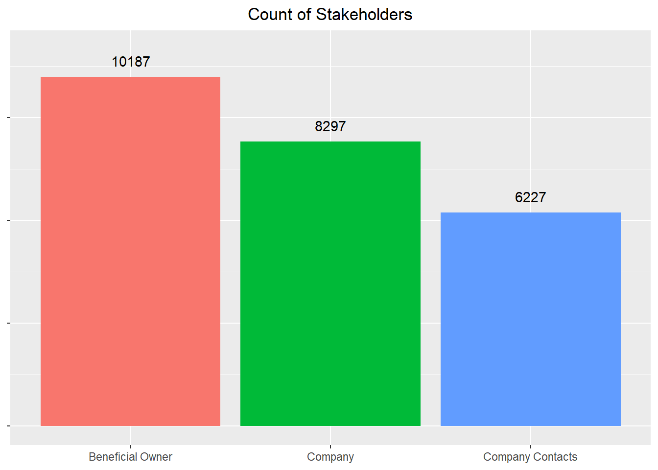
nodes_aggregated <- mc3_nodes %>%
  group_by(country, type) %>%
  summarise(count = n(),
            revenue_omu = sum(revenue_omu)) %>%
  ungroup()


pben_owner <- nodes_aggregated %>%
  filter(type == "Beneficial Owner") %>%
  ggplot(aes(x = fct_rev(fct_reorder(country, count)), y = count, fill = "Standard Color")) +
  geom_col() +
  geom_text(aes(label = count), vjust = -1) +
  ylim(0, 13000) +
  labs(title = "Beneficial Owners mostly from ZH") +
  theme(
    axis.title.y = element_blank(),
    axis.title.x = element_blank(),
    axis.text.y = element_blank(),
    legend.position = "none"
  ) +
  scale_fill_manual(values = "#F8766D")


pben_owner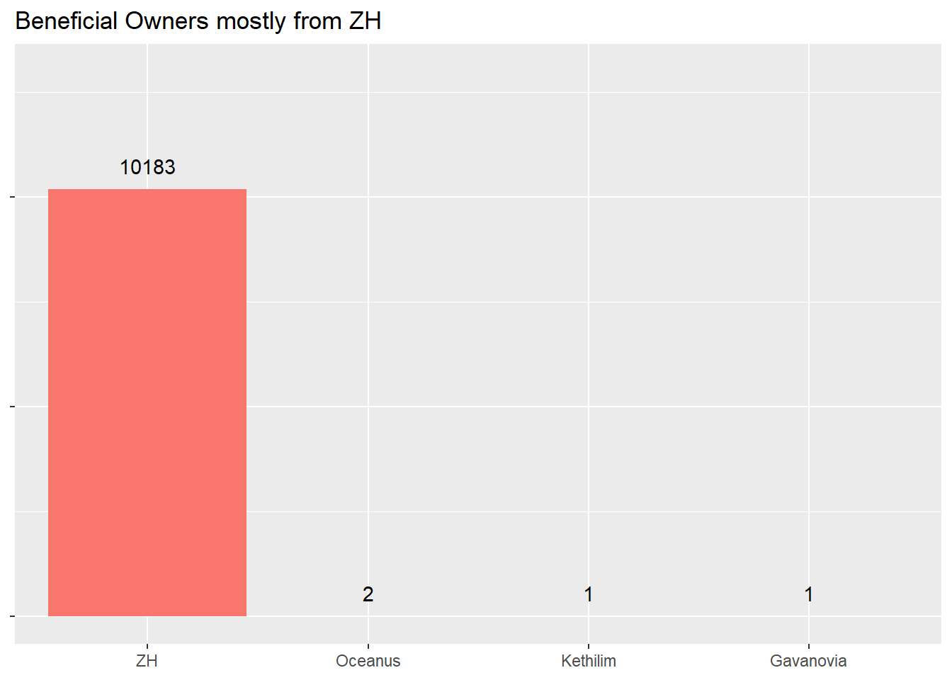
pcompany <- nodes_aggregated %>%
  filter(type == "Company" & count > 100) %>%
  ggplot(aes(x = fct_rev(fct_reorder(country, count)), y = count)) +
  geom_col(fill = "#00BA38") +
  ylim(0, 3800) +
  geom_text(aes(label = count), vjust = -1) +
  labs(title = "Companies Mostly Operating from ZH") +
  theme(
    axis.title.y = element_blank(),
    axis.title.x = element_blank(),
    axis.text.y = element_blank())


pcompany
pcoy_contacts <- nodes_aggregated %>%
  filter(type == "Company Contacts") %>%
  ggplot(aes(x = fct_rev(fct_reorder(country, count)), y = count, fill = "Standard Color")) +
  geom_col() +
  geom_text(aes(label = count), vjust = -1) +
  ylim(0, 13000) +
  labs(title = "Company Contacts mostly from ZH") +
  theme(
    axis.title.y = element_blank(),
    axis.title.x = element_blank(),
    axis.text.y = element_blank(),
    legend.position = "none"
  ) +
  scale_fill_manual(values = "#619CFF")


pcoy_contacts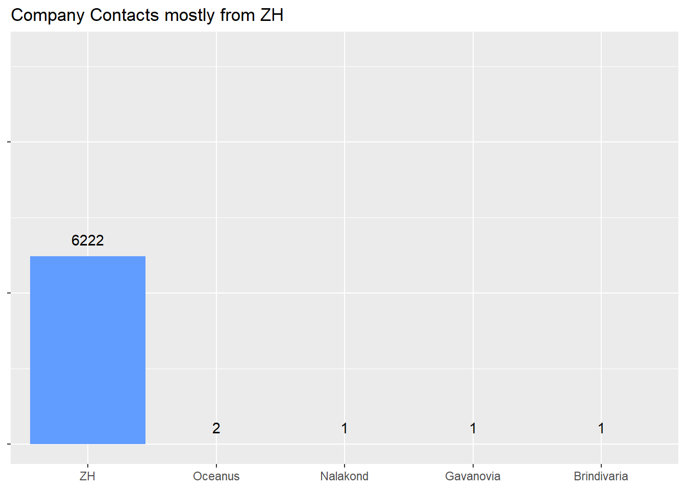
Elaborate here
1: Top 20% 2: 20 to 40% 3: 40 to 60% 4: 60 to 80% 5: Bottom 20% 6: NA
percentiles <- quantile(mc3_nodes$revenue_omu,
                        probs = c(0, 0.2, 0.4, 0.6, 0.8, 1),
                        na.rm = TRUE)

# Create a new column and assign labels based on percentiles
mc3_nodes$revenue_group <- cut(mc3_nodes$revenue_omu,
                                   breaks = percentiles,
                                   labels = c(5, 4, 3, 2, 1),
                                   include.lowest = TRUE)

company_nodes <- mc3_nodes %>%
  filter(type == "Company")

ggplot(company_nodes, aes(x = revenue_group)) +
  geom_bar(fill = "#00BA38") +
  labs(
    title = "High Number of Unreported Revenues for Companies",
    x = "Revenue Group",
    y = NULL
  ) +
  geom_text(
    stat = "count",
    aes(label = after_stat(count)),
    vjust = -1) +
  ylim(0, 10500) +
  theme(text = element_text(size = 12)) +
  facet_wrap(~type)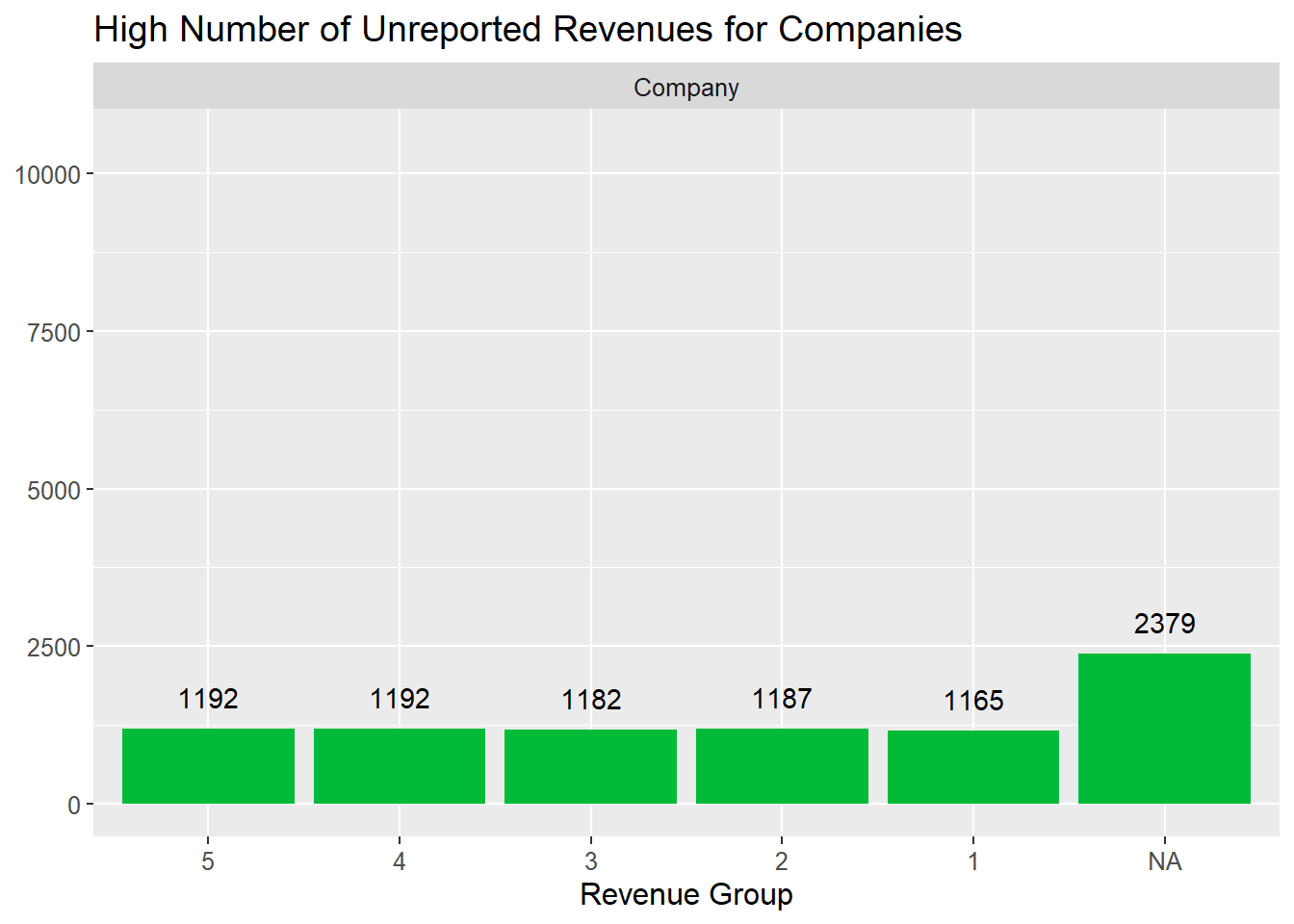
By counting the number of companies linked to each beneficial owner, we can observe which parties are linked to the highest numbers of companies at once.
target_edges <- mc3_edges_clean %>%
  group_by(target, type) %>%
  distinct() %>%
  summarise(company_count = n()) %>%
  arrange(desc(company_count)) %>%
  ungroup()

ftarget_edges <- target_edges %>%
  filter(type == "Beneficial Owner")

datatable(ftarget_edges)frequency <- table(ftarget_edges$company_count)
# Convert the frequency table to a data frame
frequency_df <- as.data.frame(frequency)
frequency_df <- frequency_df[order(frequency_df$Var1), ]
ggplot(frequency_df, aes(x = Var1, y = Freq)) +
geom_bar(stat = "identity") +
geom_text(aes(label = Freq), vjust = -0.5) +
xlab("Company Count") +
ylab("Frequency") +
ggtitle("Distribution of Companies Linked to Beneficial Owners") +
ylim(0, max(frequency_df$Freq) * 1.2)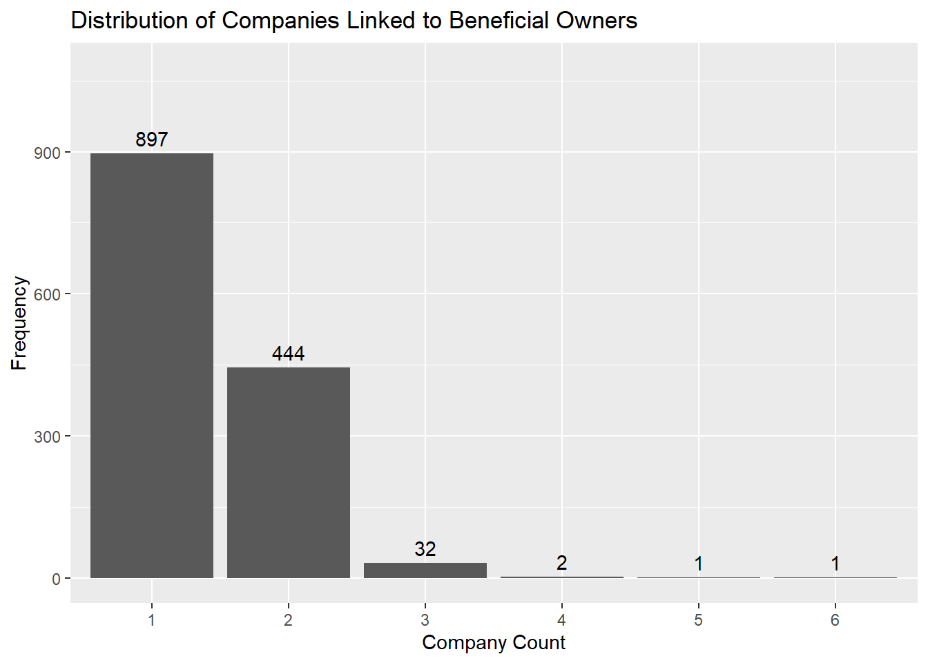
For Brevity, Beneficial Owners with >= 3 Companies will be termed Big Ben.
With the data available, there are a few possible factors to leverage on to identify anomalies.
Number of Beneficial Owners
While companies having a single Beneficial Owner is not inherently anomalous, it suggests private ownership, which provides more control, privacy and fewer regulatory requirements. It is therefore worth looking into this in combination with the following factor.
Number of Companies
While owning shares in many companies is not in itself anomalous, the nature of private ownership suggests a certain degree of privacy and freedom from regulations. As such, it is worthwhile looking into caaes of Beneficial owners with more than or equal to 3 companies [Big Bens].
Revenue
Both companies with High Revenue reported and Unreported revenue (missing values) are of interest, since these are potential signs of anomalous activity.
Products
There are companies with “Unknown” products being transacted, which could either be a data collection error, or potentially anomalous.
Therefore, we will explore the following subsets of companies:
Area of Interest 1 - Companies owned by single Beneficial Owners
Area of Interest 2 - High Revenue Companies with Big Bens
Area of Interest 3 - High Revenue Companies with Sole Big Ben
Area of Interest 4 - Companies with Large Number of Company Contacts but Undeclared Revenue.
sin_benowners <- mc3_edges_clean %>%
  group_by(source) %>%
  filter(type == "Beneficial Owner") %>%
  filter(n_distinct(target) == 1)

sin_bencount <- sin_benowners %>%
  group_by(target) %>%
  mutate(count = n()) %>%
  filter(count >= 3) %>%
  ungroup()


sin_bencount_rev <- left_join(sin_bencount, mc3_nodes, by = c("source"="id")) %>%
  select(-type.y) %>%
  rename("type" = "type.x")

sin_bencount_rev2 <-  sin_bencount_rev %>%
  distinct() %>%
  rename("from" = "source",
         "to" = "target")

benowner_source <- sin_bencount_rev2 %>%
  distinct(from) %>%
  rename("id" = "from")

benowner_target <- sin_bencount_rev2 %>%
  distinct(to) %>%
  rename("id" = "to")

benowner_nodes_extracted <- rbind(benowner_source, benowner_target)

benowner_nodes_extracted$group <- ifelse(benowner_nodes_extracted$id %in% sin_bencount_rev$source, "Company", "Beneficial Owner")visNetwork(
benowner_nodes_extracted,
sin_bencount_rev2,
width = "100%",
main = list(
text = "Anna Wheeler is the sole Beneficial Owner",
style = "font-size:17x; weight:bold; text-align:right;"),
submain = list(text = "of 6 different Companies",
style = "font-size:13pm;
text-align:right;")
)%>%
visIgraphLayout(
layout = "layout_with_fr"
) %>%
visGroups(groupname = "Company",
color = "#00BA38") %>%
visGroups(groupname = "Beneficial Owner",
color = "#F8766D") %>%
visLegend() %>%
visEdges(
arrows = "to"
) %>%
visOptions(
highlightNearest = list(enabled = T, degree = 2, hover = T),
nodesIdSelection = TRUE,
selectedBy = "group",
collapse = TRUE)General Findings
With multiple Beneficial Owners typically signalling a company being in the public domain as a publicly listed company, sole ownership typically signals that a company is privately owned. Privately owned companies enjoy privileges that publicly listed companies do not: privacy, and less regulations.
As such, it is far more accessible for Beneficial Owners who are the sole owners of companies to utilise their various assets and connections to mask illegal activities whilst being poorly regulated by the industry officials. It is therefore worth monitoring and looking into these individuals.
hr_nodes <- company_nodes %>%
  filter(revenue_group == "1")

target_3 <- ftarget_edges[ftarget_edges$company_count >= 3, ]

hr_edges <- mc3_edges_clean %>%
  filter(source %in% hr_nodes$id) %>%
  filter(target %in% target_3$target) %>%
  rename(from = source, to = target) %>%
  distinct()

hr_nodes_extract <- hr_edges %>%
  select(from) %>%
  rename(id = from) %>%
  bind_rows(hr_edges %>%
              select(to) %>%
              rename(id = to)) %>%
  distinct() %>%
mutate(group = ifelse(id %in% hr_edges$from, "Company", "Beneficial Owner"))# Define the color palette
visNetwork(
hr_nodes_extract,
hr_edges,
width = "100%",
main = list(
text = "Primarily Private Ownership except for",
style = "font-size:17x; weight:bold; text-align:right;"),
submain = list(text = "Mar de la Aventura Tidepool",
style = "font-size:13pm;
text-align:right;")
) %>%
visIgraphLayout(layout = "layout_nicely") %>%
visGroups(groupname = "Company", color = "#00BA38") %>%
visGroups(groupname = "Beneficial Owner", color = "#F8766D") %>%
visLegend() %>%
visEdges(arrows = "to") %>%
visOptions(
highlightNearest = list(enabled = TRUE, degree = 2, hover = TRUE),
nodesIdSelection = TRUE,
selectedBy = "group",
collapse = TRUE
) %>%
visInteraction(navigationButtons = TRUE)General Findings
Having filtered the dataset to detect for the specific links between Beneficial Owners with links to >= 3 companies, and Companies in the top revenue group, we can make the following observations:
Mar de la Aventura presents itself as a potential publicly listed company that produces high revenue with multiple Big Bens.
Conversely, there are also cases where these Owners are the only one among their population to have stakes in Company within the top income revenue group. However, this does not shed much light on the specific group of companies/owners of interest, as this network graph could have excluded other owners who do not own multiple businesses.
We therefore include another filter where we match the companies to a list of companies with only one Beneficial Owner.
companies_with_one_owner <- hr_edges %>%
  group_by(from) %>%
  summarise(count = n()) %>%
  filter(count == 1)

excl_hredges <- hr_edges %>%
  filter(from %in% companies_with_one_owner$from)


excl_hrnodes_extract <- excl_hredges %>%
  select(from) %>%
  rename(id = from) %>%
  bind_rows(excl_hredges %>%
              select(to) %>%
              rename(id = to)) %>%
  distinct() %>%
mutate(group = ifelse(id %in% excl_hredges$from, "Company", "Beneficial Owner"))visNetwork(
excl_hrnodes_extract,
excl_hredges,
width = "100%",
main = list(
text = "Tiffany Brown and John Williams solely own",
style = "font-size:17x; weight:bold; text-align:right;"),
submain = list(text = "two High Revenue companies respectively",
style = "font-size:13pm;
text-align:right;")
) %>%
visIgraphLayout(layout = "layout_nicely") %>%
visGroups(groupname = "Company", color = "#00BA38") %>%
visGroups(groupname = "Beneficial Owner", color = "#F8766D") %>%
visLegend() %>%
visEdges(arrows = "to") %>%
visOptions(
highlightNearest = list(enabled = TRUE, degree = 2, hover = TRUE),
nodesIdSelection = TRUE,
selectedBy = "group",
collapse = TRUE
) %>%
visInteraction(navigationButtons = TRUE)General Findings
This specific subset of Companies x Beneficial Owners is worth looking into because both groups belong to an exclusive list of companies that are in the top revenue group, while having just one Beneficial Owner who owns multiple companies. In two particular instances, we see Tiffany Brown and John Williams being the sole owners of two top performing companies at the same time.
Though not particularly incriminating, it is worth looking into these individuals and their companies to monitor for any illicit activities that may be facilitating their high revenue across multiple companies.
#Added after deadline to value-add

# Assuming your dataset is named 'data'
sus_edges <- subset(mc3_edges_clean, target %in% c("Tiffany Brown", "John Williams"))

colnames(sus_edges)[colnames(sus_edges) == "source"] <- "from"
colnames(sus_edges)[colnames(sus_edges) == "target"] <- "to"

sus_nodes_extract <- sus_edges %>%
  select(from) %>%
  rename(id = from) %>%
  bind_rows(sus_edges %>%
              select(to) %>%
              rename(id = to)) %>%
  distinct() %>%
  mutate(group = ifelse(id %in% sus_edges$from, "Company", "Beneficial Owner"))

visNetwork(
  sus_nodes_extract,
  sus_edges,
  width = "100%",
  main = list(
    text = "Companies owned by Tiffany Brown and John Williams",
    style = "font-size:17x; weight:bold; text-align:right;")) %>%
visIgraphLayout(layout = "layout_nicely") %>%
visGroups(groupname = "Company", color = "#00BA38") %>%
visGroups(groupname = "Beneficial Owner", color = "#F8766D") %>%
visLegend() %>%
visEdges(arrows = "to") %>%
visOptions(
  highlightNearest = list(enabled = TRUE, degree = 2, hover = TRUE),
  nodesIdSelection = TRUE,
  selectedBy = "group",
  collapse = TRUE
) %>%
visInteraction(navigationButtons = TRUE)
Additional Findings
It is observed that Tiffany Brown and John Williams are also sole owners of other companies.
It might be worth looking into these companies in the event they may be shell companies.
cc_edges <- mc3_edges_clean %>%
  group_by(target, type) %>%
  distinct() %>%
  summarise(contacts_count = n()) %>%
  arrange(desc(contacts_count)) %>%
  ungroup()

fcc_edges <- cc_edges %>%
  filter(type == "Company Contacts")

datatable(fcc_edges)ccfrequency <- table(fcc_edges$contacts_count)
# Convert the frequency table to a data frame
ccfrequency_df <- as.data.frame(ccfrequency)
ccfrequency_df <- ccfrequency_df[order(ccfrequency_df$Var1), ]
ggplot(ccfrequency_df, aes(x = Var1, y = Freq)) +
geom_bar(stat = "identity") +
geom_text(aes(label = Freq), vjust = -0.5) +
xlab("Contacts Count") +
ylab("Frequency") +
ggtitle("Distribution of Companies Contacts linked to Companies") +
ylim(0, max(frequency_df$Freq) * 1.2)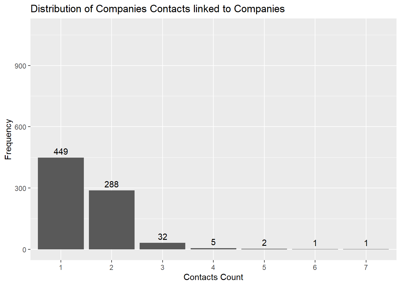
Most companies have 1-2 Company Contacts, which makes companies with 3 or more contacts an anomaly. To further the discrepancy, we will specifically look into companies with >= 3 contacts (which suggest larger size and potential revenue) and yet have undisclosed revenues.
udrev_nodes <- mc3_nodes %>%
  filter(is.na(revenue_omu))

udrev_nodes_cc <- udrev_nodes %>%
  filter(type == "Company Contacts") %>%
  distinct()


udrev_edges <- mc3_edges %>%
  filter(type == "Company Contacts") %>%
  filter(source %in% udrev_nodes_cc$id) %>%
  distinct() %>%
  rename("from" = "source",
         "to" = "target")

# Extract edges that have more than or equal to 3 company contacts
high_udrev_edges <- udrev_edges %>%
  group_by(from) %>%
  mutate(count = n()) %>%
  filter(count >= 3) %>%
  ungroup()


udrev_source <- high_udrev_edges %>%
  distinct(from) %>%
  rename("id" = "from")

udrev_target <- high_udrev_edges %>%
  distinct(to) %>%
  rename("id" = "to")

# Bind into one dataframe
udrev_nodes2 <- bind_rows(udrev_source, udrev_target)

udrev_nodes2$group <- ifelse(udrev_nodes2$id %in% udrev_nodes_cc$id, "Company Contact", "Company")visNetwork(
udrev_nodes2,
high_udrev_edges
) %>%
visIgraphLayout(
layout = "layout_with_fr"
) %>%
visGroups(groupname = "Company",
color = "#00BA38") %>%
visGroups(groupname = "Company Contact",
color = "#619CFF") %>%
visLegend() %>%
visEdges(
arrows = "to"
) %>%
visOptions(
highlightNearest = list(enabled = T, degree = 2, hover = T),
nodesIdSelection = TRUE,
selectedBy = "group",
collapse = TRUE)While absent data for revenue is not an immediate justification to label these companies as participating in illegal activities, the noted lack of revenue being declared coupled with their suggested size (inconclusive without more information) warrants deeper investigation and monitoring.
Delving into the distribution and spread of factors such as revenue and ownership has provided insights that have been explored through basic graph and network graph visualisations. While certain anomalous areas were detected, there is insufficient data to conclusively identify any individual(s) or company participating in illegal activities.
Further work may include standardisation of product service categories/keywords so that the data can be cleanly segmented by product type. It would also be helpful if companies are labeled private/public to begin with, that we may compare within each category.