Show me the good stuff
pacman::p_load(igraph, tidygraph, ggraph,
               visNetwork, lubridate, clock,
tidyverse, graphlayouts, jsonlite)pacman::p_load(igraph, tidygraph, ggraph,
visNetwork, lubridate, clock,
tidyverse, graphlayouts, jsonlite)MC1 <- fromJSON("data/MC1.json")
GAStech_nodes <- read_csv("data/GAStech_email_node.csv")
GAStech_edges <- read_csv("data/GAStech_email_edge-v2.csv")MC1_nodes <- as_tibble(MC1$nodes) %>%
select(id, type, country) #using select function to reorganise into desired order of columnsMC1_edges <- as_tibble(MC1$links) %>%
select(source, target, type, weight, key)glimpse(GAStech_edges)Rows: 9,063
Columns: 8
$ source <dbl> 43, 43, 44, 44, 44, 44, 44, 44, 44, 44, 44, 44, 26, 26, 26…
$ target <dbl> 41, 40, 51, 52, 53, 45, 44, 46, 48, 49, 47, 54, 27, 28, 29…
$ SentDate <chr> "6/1/2014", "6/1/2014", "6/1/2014", "6/1/2014", "6/1/2014"…
$ SentTime <time> 08:39:00, 08:39:00, 08:58:00, 08:58:00, 08:58:00, 08:58:0…
$ Subject <chr> "GT-SeismicProcessorPro Bug Report", "GT-SeismicProcessorP…
$ MainSubject <chr> "Work related", "Work related", "Work related", "Work rela…
$ sourceLabel <chr> "Sven.Flecha", "Sven.Flecha", "Kanon.Herrero", "Kanon.Herr…
$ targetLabel <chr> "Isak.Baza", "Lucas.Alcazar", "Felix.Resumir", "Hideki.Coc…GAStech_edges <- GAStech_edges %>%
mutate(SendDate = dmy(SentDate)) %>%
mutate(Weekday = wday(SentDate,
label = TRUE,
abbr = FALSE))
glimpse(GAStech_edges) #Review dataRows: 9,063
Columns: 10
$ source <dbl> 43, 43, 44, 44, 44, 44, 44, 44, 44, 44, 44, 44, 26, 26, 26…
$ target <dbl> 41, 40, 51, 52, 53, 45, 44, 46, 48, 49, 47, 54, 27, 28, 29…
$ SentDate <chr> "6/1/2014", "6/1/2014", "6/1/2014", "6/1/2014", "6/1/2014"…
$ SentTime <time> 08:39:00, 08:39:00, 08:58:00, 08:58:00, 08:58:00, 08:58:0…
$ Subject <chr> "GT-SeismicProcessorPro Bug Report", "GT-SeismicProcessorP…
$ MainSubject <chr> "Work related", "Work related", "Work related", "Work rela…
$ sourceLabel <chr> "Sven.Flecha", "Sven.Flecha", "Kanon.Herrero", "Kanon.Herr…
$ targetLabel <chr> "Isak.Baza", "Lucas.Alcazar", "Felix.Resumir", "Hideki.Coc…
$ SendDate <date> 2014-01-06, 2014-01-06, 2014-01-06, 2014-01-06, 2014-01-0…
$ Weekday <ord> Friday, Friday, Friday, Friday, Friday, Friday, Friday, Fr…GAStech_edges_aggregated <- GAStech_edges %>%
filter(MainSubject == "Work related") %>%
group_by(source, target, Weekday) %>%
summarise(Weight = n()) %>%
filter(source!=target) %>%
filter(Weight > 1) %>%
ungroup()
glimpse(GAStech_edges_aggregated)Rows: 1,372
Columns: 4
$ source <dbl> 1, 1, 1, 1, 1, 1, 1, 1, 1, 1, 1, 1, 1, 1, 1, 1, 1, 1, 1, 1, 1,…
$ target <dbl> 2, 2, 2, 2, 2, 3, 3, 3, 3, 3, 4, 4, 4, 4, 4, 5, 5, 5, 5, 5, 6,…
$ Weekday <ord> Sunday, Monday, Tuesday, Wednesday, Friday, Sunday, Monday, Tu…
$ Weight <int> 5, 2, 3, 4, 6, 5, 2, 3, 4, 6, 5, 2, 3, 4, 6, 5, 2, 3, 4, 6, 5,…GAStech_graph <- tbl_graph(nodes = GAStech_nodes,
edges = GAStech_edges_aggregated,
directed = TRUE)
GAStech_graph #Review Graph# A tbl_graph: 54 nodes and 1372 edges
#
# A directed multigraph with 1 component
#
# A tibble: 54 × 4
id label Department Title
<dbl> <chr> <chr> <chr>
1 1 Mat.Bramar Administration Assistant to CEO
2 2 Anda.Ribera Administration Assistant to CFO
3 3 Rachel.Pantanal Administration Assistant to CIO
4 4 Linda.Lagos Administration Assistant to COO
5 5 Ruscella.Mies.Haber Administration Assistant to Engineering Group Manag…
6 6 Carla.Forluniau Administration Assistant to IT Group Manager
# ℹ 48 more rows
#
# A tibble: 1,372 × 4
from to Weekday Weight
<int> <int> <ord> <int>
1 1 2 Sunday 5
2 1 2 Monday 2
3 1 2 Tuesday 3
# ℹ 1,369 more rowsGAStech_graph %>%
activate(edges) %>%
arrange(desc(Weight))# A tbl_graph: 54 nodes and 1372 edges
#
# A directed multigraph with 1 component
#
# A tibble: 1,372 × 4
from to Weekday Weight
<int> <int> <ord> <int>
1 40 41 Saturday 13
2 41 43 Monday 11
3 35 31 Tuesday 10
4 40 41 Monday 10
5 40 43 Monday 10
6 36 32 Sunday 9
# ℹ 1,366 more rows
#
# A tibble: 54 × 4
id label Department Title
<dbl> <chr> <chr> <chr>
1 1 Mat.Bramar Administration Assistant to CEO
2 2 Anda.Ribera Administration Assistant to CFO
3 3 Rachel.Pantanal Administration Assistant to CIO
# ℹ 51 more rowsggraph(GAStech_graph) +
geom_edge_link() +
geom_node_point()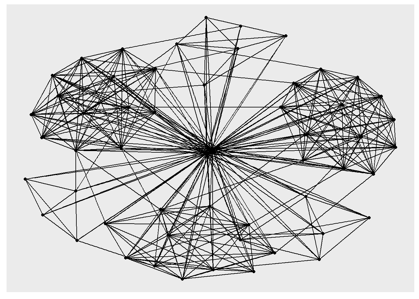
The basic plotting function is ggraph(), which takes the data to be used for the graph and the type of layout desired. Both of the arguments for ggraph() are built around igraph. Therefore, ggraph() can use either an igraph object or a tbl_graph object.
g <- ggraph(GAStech_graph) +
  geom_edge_link(aes()) +
  geom_node_point(aes())

g + theme_graph()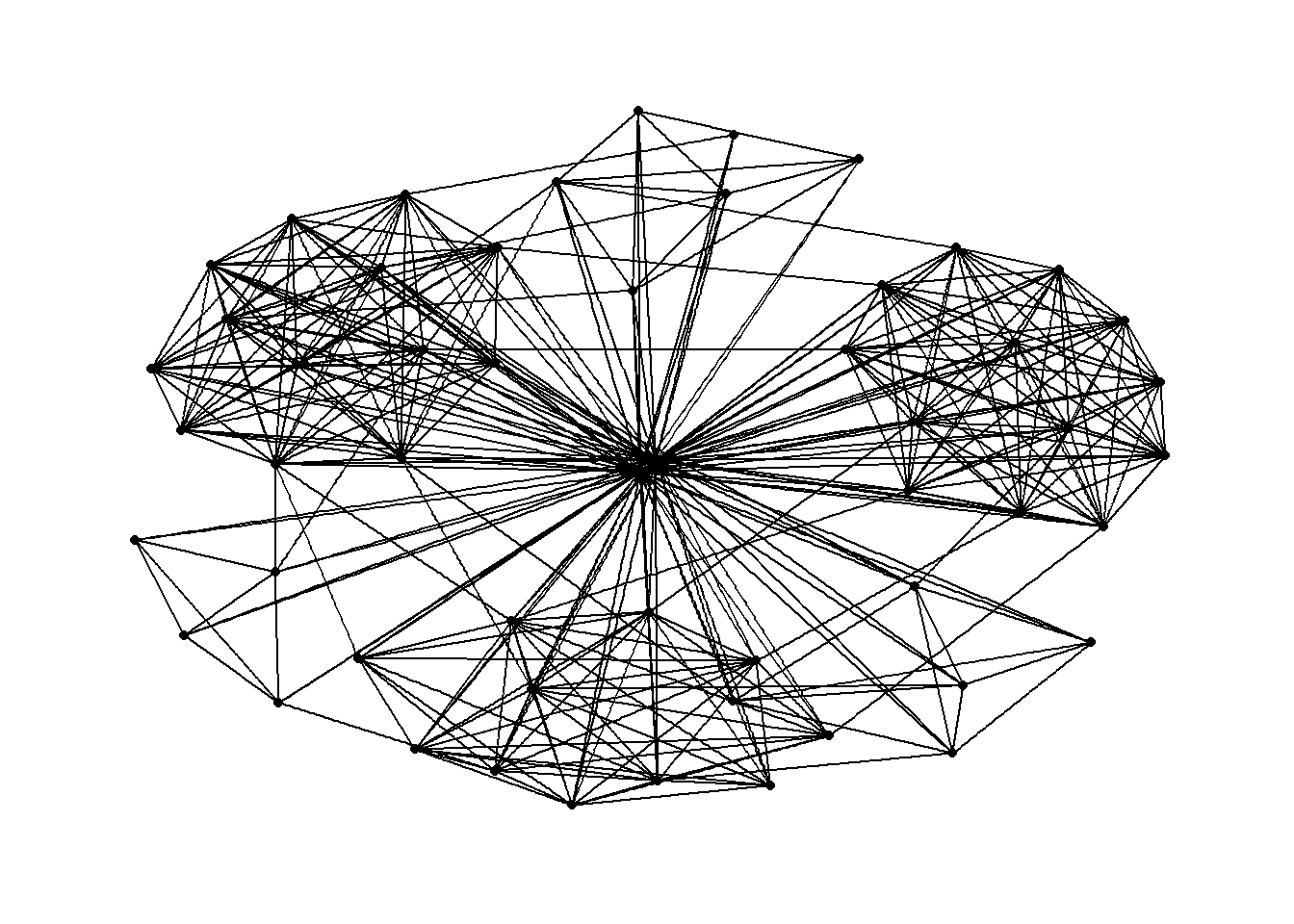
g <- ggraph(GAStech_graph) +
  geom_edge_link(aes(colour = 'grey50')) +
  geom_node_point(aes(colour = 'grey40'))

g + theme_graph(background = 'grey10',
                text_colour = 'white')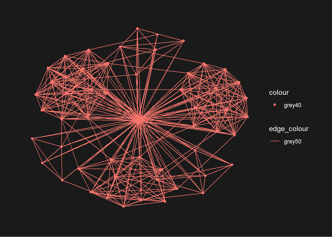
g <- ggraph(GAStech_graph,
            layout = "fr") +
  geom_edge_link(aes()) +
  geom_node_point(aes())

g + theme_graph()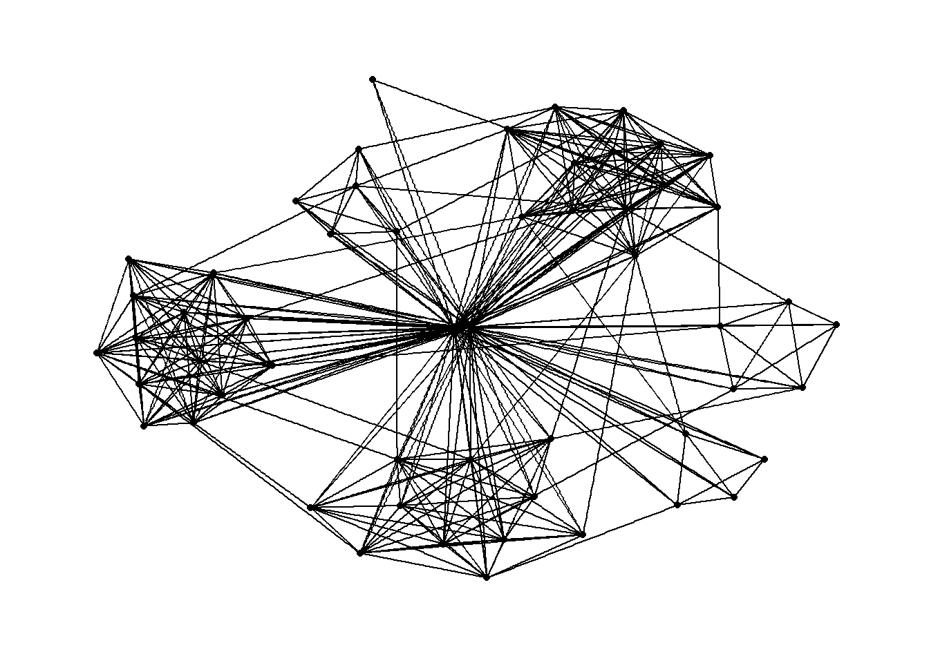
g <- ggraph(GAStech_graph,
            layout = "nicely") +
  geom_edge_link(aes()) +
  geom_node_point(aes(colour = Department,
                      size = 3))

g + theme_graph()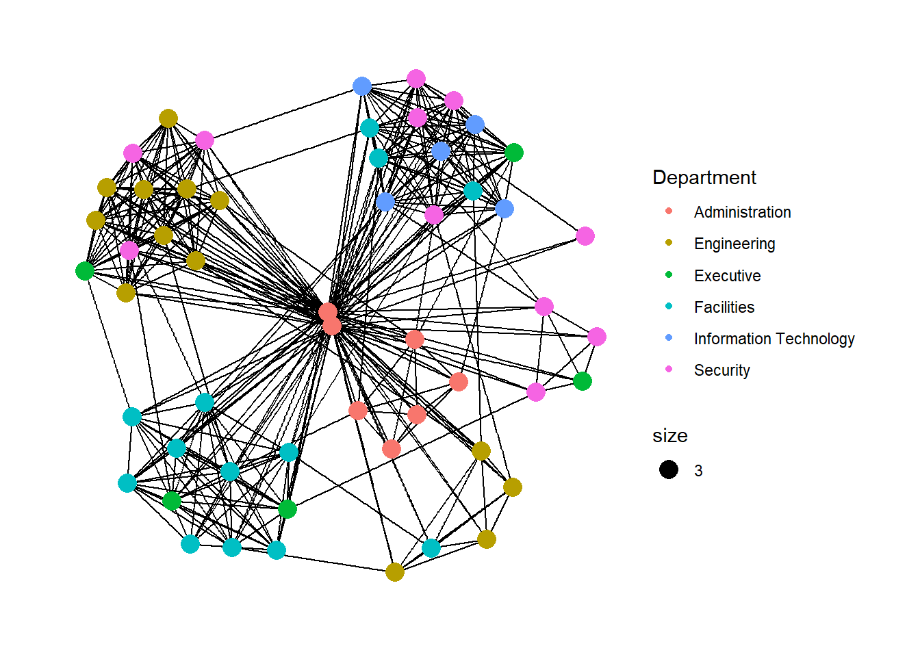
geom_node_point is equivalent in functionality to geo_point of ggplot2. It allows for simple plotting of nodes in different shapes, colours and sizes. In the codes chnuks above colour and size are used.
g <- ggraph(GAStech_graph,
            layout = "nicely") +
  geom_edge_link(aes(width=Weight),
                 alpha=0.2) +
  scale_edge_width(range = c(0.1, 5)) +
  geom_node_point(aes(colour = Department),
                  size = 3)

g + theme_graph()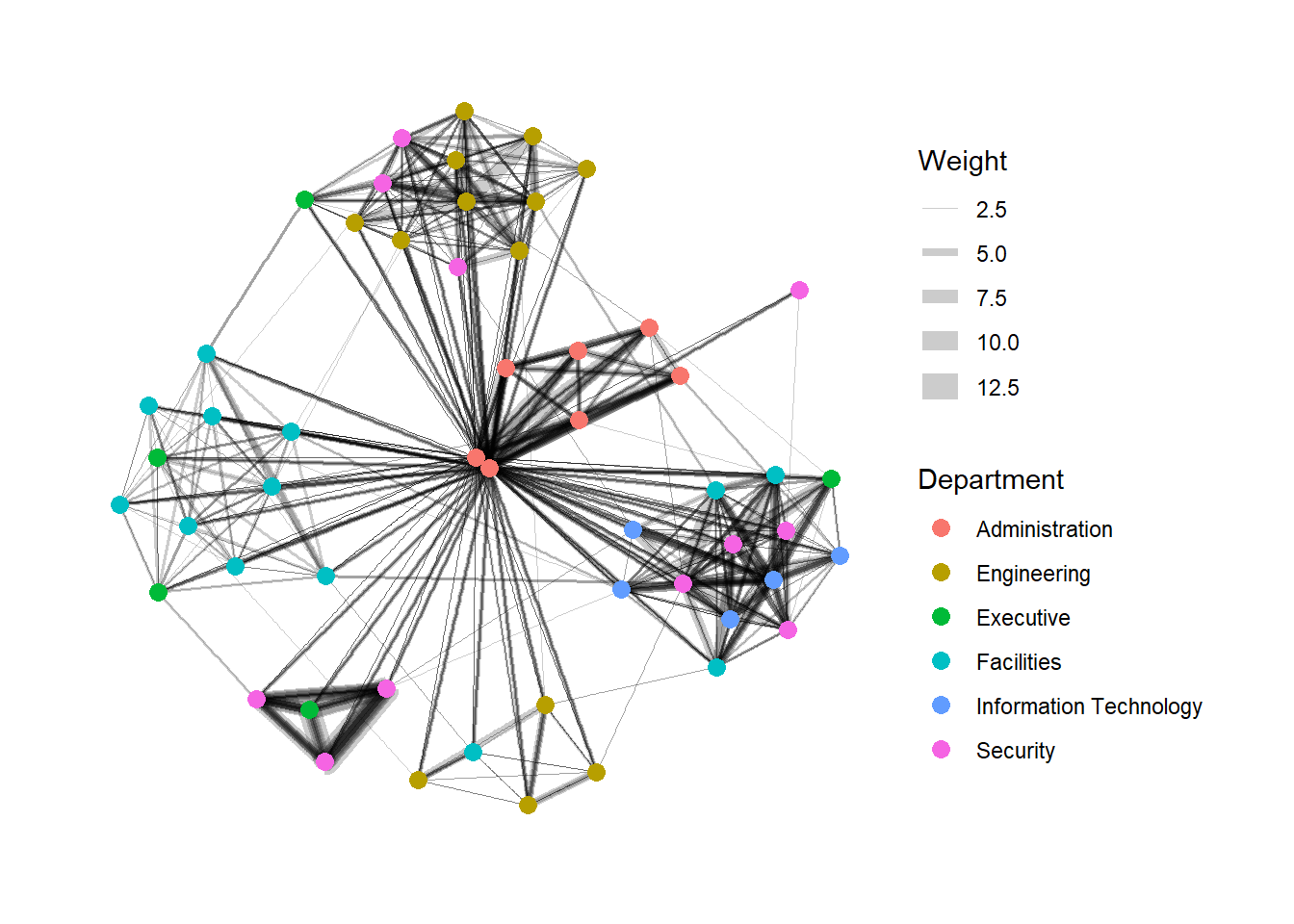
There are three functions in ggraph to implement faceting, they are:
facet_nodes() whereby edges are only draw in a panel if both terminal nodes are present here, facet_edges() whereby nodes are always drawn in al panels even if the node data contains an attribute named the same as the one used for the edge facetting, and facet_graph() faceting on two variables simultaneously.
set_graph_style()

g <- ggraph(GAStech_graph,
            layout = "nicely") +
  geom_edge_link(aes(width=Weight),
                 alpha=0.2) +
  scale_edge_width(range = c(0.1, 5)) +
  geom_node_point(aes(colour = Department),
                  size = 2)

g + facet_edges(~Weekday)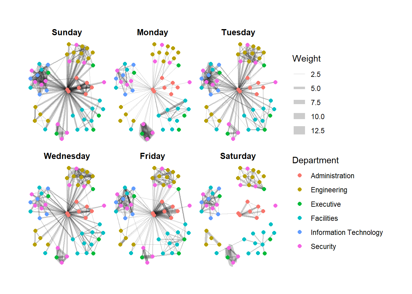
set_graph_style()

g <- ggraph(GAStech_graph,
            layout = "nicely") +
  geom_edge_link(aes(width=Weight),
                 alpha=0.2) +
  scale_edge_width(range = c(0.1, 5)) +
  geom_node_point(aes(colour = Department),
                  size = 2) +
  theme(legend.position = 'bottom')

g + facet_edges(~Weekday)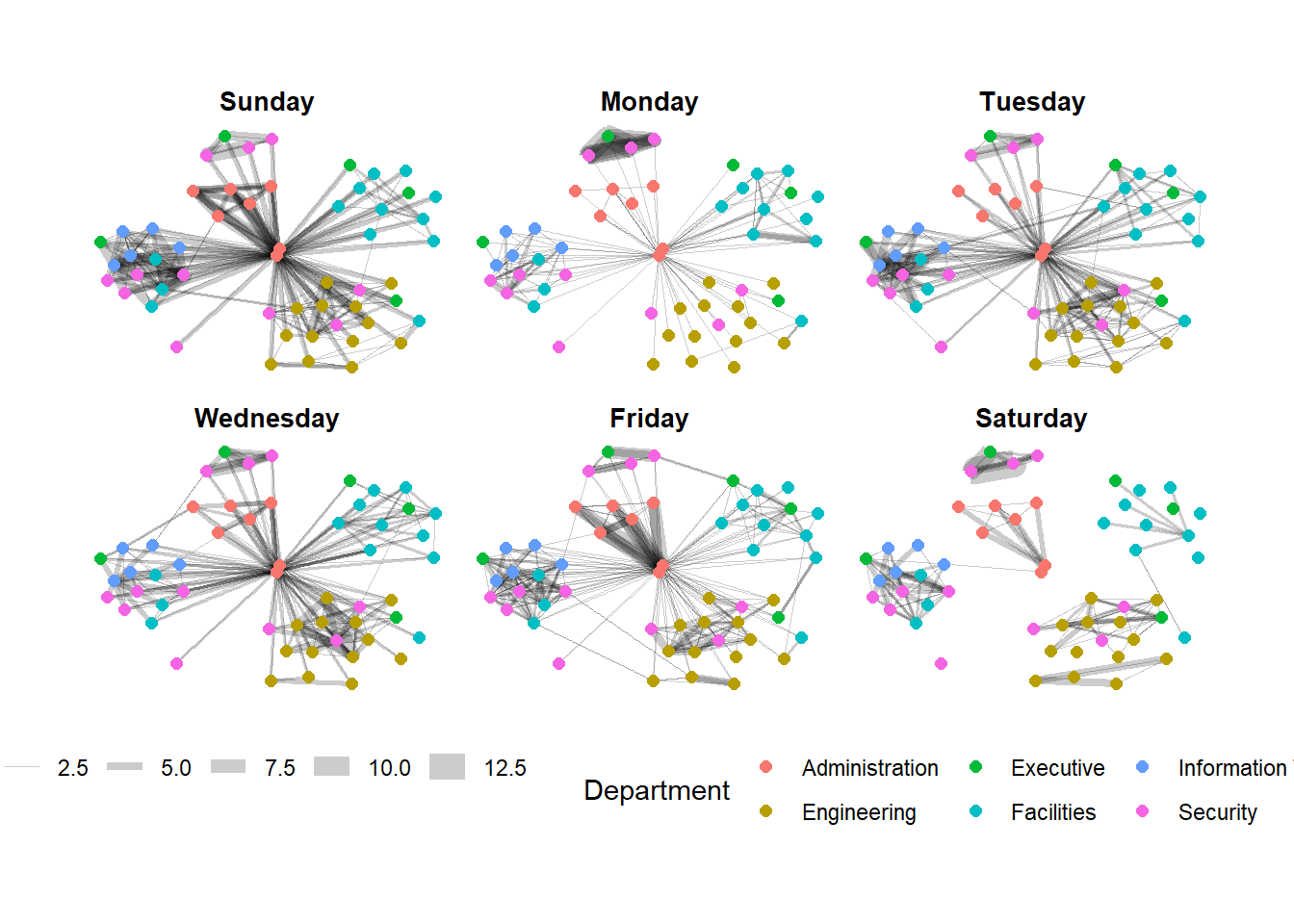
set_graph_style()

g <- ggraph(GAStech_graph,
            layout = "nicely") +
  geom_edge_link(aes(width=Weight),
                 alpha=0.2) +
  scale_edge_width(range = c(0.1, 5)) +
  geom_node_point(aes(colour = Department),
                  size = 2)

g + facet_edges(~Weekday) +
  th_foreground(foreground = "grey80",
                border = TRUE) +
  theme(legend.position = 'bottom')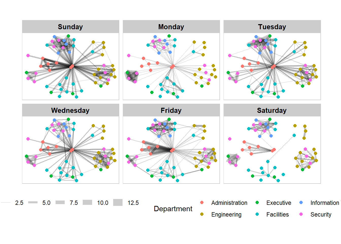
set_graph_style()

g <- ggraph(GAStech_graph,
            layout = "nicely") +
  geom_edge_link(aes(width=Weight),
                 alpha=0.2) +
  scale_edge_width(range = c(0.1, 5)) +
  geom_node_point(aes(colour = Department),
                  size = 2)

g + facet_nodes(~Department)+
  th_foreground(foreground = "grey80",
                border = TRUE) +
  theme(legend.position = 'bottom')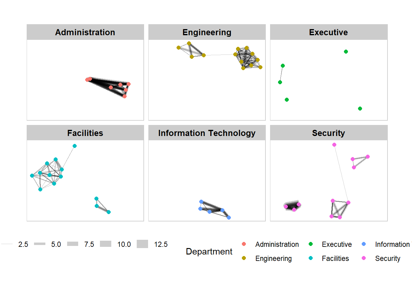
Centrality measures are a collection of statistical indices use to describe the relative important of the actors are to a network. There are four well-known centrality measures, namely: degree, betweenness, closeness and eigenvector.
g <- GAStech_graph %>%
  mutate(betweenness_centrality = centrality_betweenness()) %>%
  ggraph(layout = "fr") +
  geom_edge_link(aes(width=Weight),
                 alpha=0.2) +
  scale_edge_width(range = c(0.1, 5)) +
  geom_node_point(aes(colour = Department,
            size=betweenness_centrality))
g + theme_graph()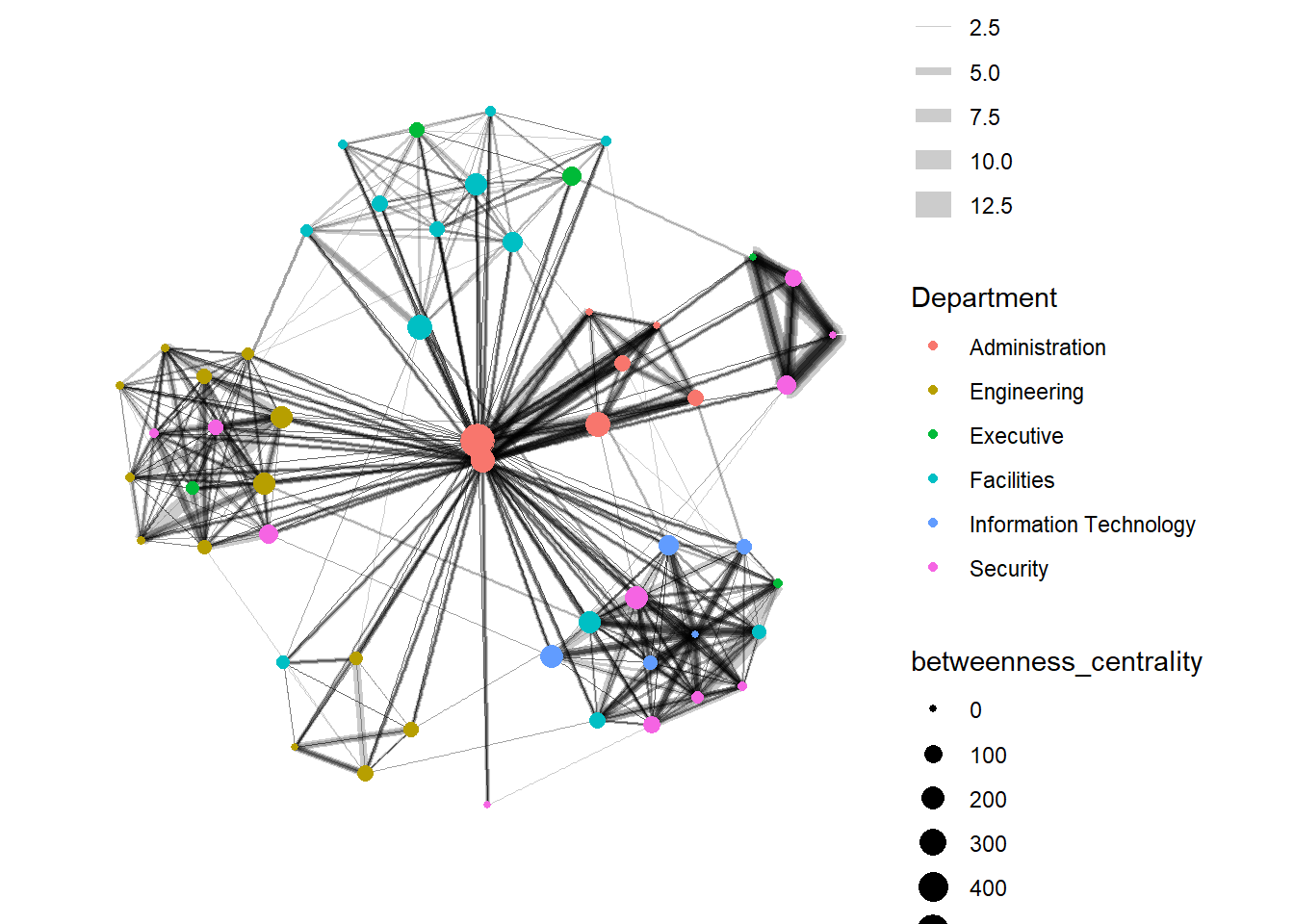
g <- GAStech_graph %>%
  ggraph(layout = "fr") +
  geom_edge_link(aes(width=Weight),
                 alpha=0.2) +
  scale_edge_width(range = c(0.1, 5)) +
  geom_node_point(aes(colour = Department,
                      size = centrality_betweenness()))
g + theme_graph()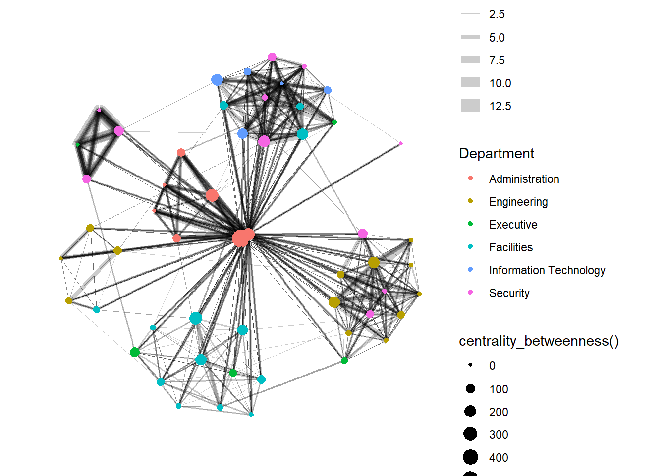
g <- GAStech_graph %>%
  mutate(community = as.factor(group_edge_betweenness(weights = Weight, directed = TRUE))) %>%
  ggraph(layout = "fr") +
  geom_edge_link(aes(width=Weight),
                 alpha=0.2) +
  scale_edge_width(range = c(0.1, 5)) +
  geom_node_point(aes(colour = community))

g + theme_graph()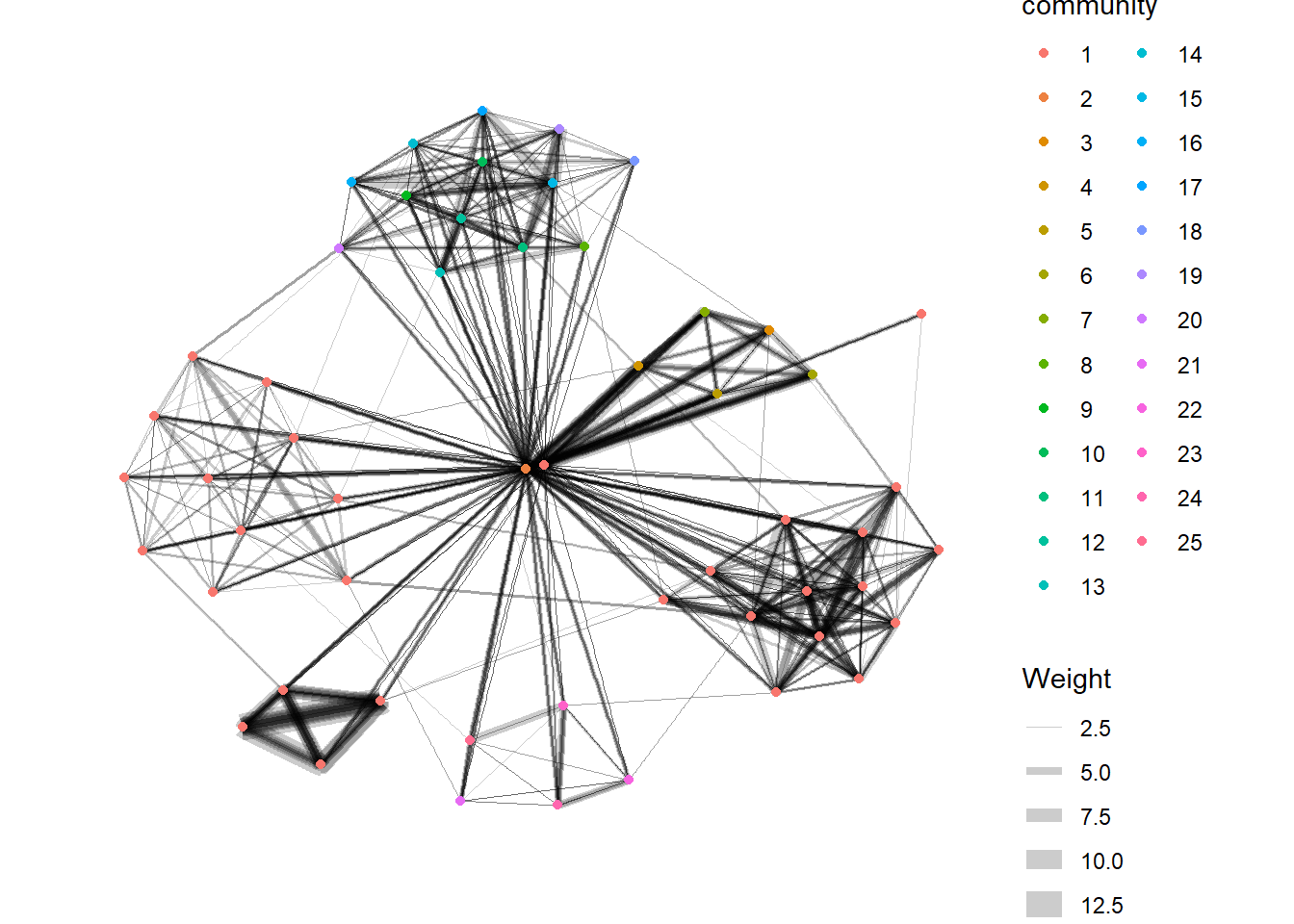
visNetwork() is a R package for network visualization, using vis.js javascript library.
visNetwork() function uses a nodes list and edges list to create an interactive graph.
The nodes list must include an “id” column, and the edge list must have “from” and “to” columns. The function also plots the labels for the nodes, using the names of the actors from the “label” column in the node list. The resulting graph is fun to play around with.
You can move the nodes and the graph will use an algorithm to keep the nodes properly spaced. You can also zoom in and out on the plot and move it around to re-center it.
GAStech_edges_aggregated <- GAStech_edges %>%
  left_join(GAStech_nodes, by = c("sourceLabel" = "label")) %>%
  rename(from = id) %>%
  left_join(GAStech_nodes, by = c("targetLabel" = "label")) %>%
  rename(to = id) %>%
  filter(MainSubject == "Work related") %>%
  group_by(from, to) %>%
    summarise(weight = n()) %>%
  filter(from!=to) %>%
  filter(weight > 1) %>%
ungroup()visNetwork(GAStech_nodes,
GAStech_edges_aggregated)visNetwork(GAStech_nodes,
GAStech_edges_aggregated) %>%
visIgraphLayout(layout = "layout_with_fr") visNetwork() looks for a field called “group” in the nodes object and colour the nodes according to the values of the group field.
The code chunk below rename Department field to group.
GAStech_nodes <- GAStech_nodes %>%
rename(group = Department) When we rerun the code chunk below, visNetwork shades the nodes by assigning unique colour to each category in the group field.
visNetwork(GAStech_nodes,
GAStech_edges_aggregated) %>%
visIgraphLayout(layout = "layout_with_fr") %>%
visLegend() %>%
visLayout(randomSeed = 123)In the code run below visEdges() is used to symbolise the edges. - The argument arrows is used to define where to place the arrow. - The smooth argument is used to plot the edges using a smooth curve.
visNetwork(GAStech_nodes,
           GAStech_edges_aggregated) %>%
visIgraphLayout(layout = "layout_with_fr") %>%
visEdges(arrows = "to",
smooth = list(enabled = TRUE,
type = "curvedCW")) %>%
visLegend() %>%
visLayout(randomSeed = 123)visNetwork(GAStech_nodes,
GAStech_edges_aggregated) %>%
visIgraphLayout(layout = "layout_with_fr") %>%
visOptions(highlightNearest = TRUE,
nodesIdSelection = TRUE) %>%
visLegend() %>%
visLayout(randomSeed = 123)